Problem
As the old saying goes, money doesn’t buy happiness. For the sake of this example, let’s say that researchers in both Canada and Mexico independently collected data to test the saying. Each group found that their citizens’ happiness ratings decrease uniformly as income increases. It may appear, then, that the saying is true: the more money you get, the less happy you will be. In other words, there is a negative correlation between money and happiness. However, when you aggregate, or combine, the data from Canada and Mexico into one evaluation, the opposite is true. The average Canadian makes significantly more money than the average Mexican, so their average happiness ratings start at a higher level in conjunction with their higher income. So, Mexicans, on average, make less money and are less happy, while Canadians, on average, make more money and are happier. Put these two together, and a positive correlation between money and happiness appears. Therefore, to a certain extent, money does buy happiness.
The Answer
Different patterns can be observed from the same set of data depending on how it is partitioned, or separated. The two variables in this hypothetical, money and happiness, have a negative correlation when considered separately for Mexico and Canada. But when they are analyzed together, they have a positive correlation.
Simpson’s Paradox
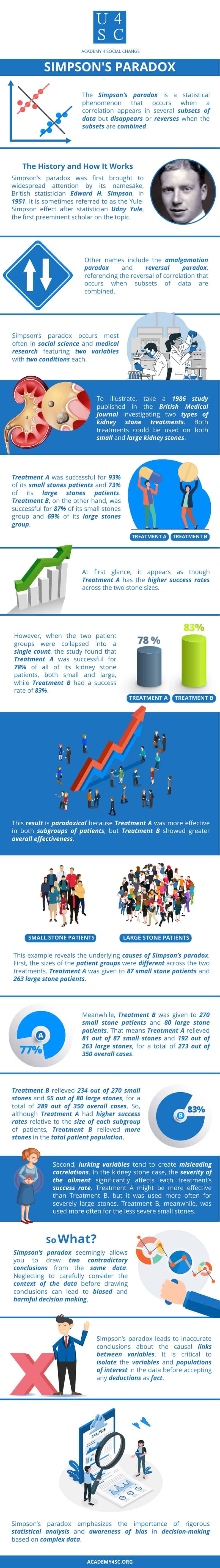
This is an example of Simpson’s paradox, a statistical phenomenon that occurs when a correlation appears in several subsets of data but disappears or reverses when the subsets are combined.
The History and How It Works
Simpson’s paradox was first brought to widespread attention by its namesake, British statistician Edward H. Simpson, in 1951. It is sometimes referred to as the Yule-Simpson effect after statistician Udny Yule, the first preeminent scholar on the topic. Other names include the amalgamation paradox and reversal paradox, referencing the reversal of correlation that occurs when subsets of data are combined.
Simpson’s paradox occurs most often in social science and medical research featuring two variables with two conditions each. To illustrate, take a 1986 study published in the British Medical Journal investigating two types of kidney stone treatments. Both treatments could be used on both small and large kidney stones. Treatment A was successful for 93% of its small stones patients and 73% of its large stones patients. Treatment B, on the other hand, was successful for 87% of its small stones group and 69% of its large stones group. At first glance, it appears as though Treatment A has the higher success rates across the two stone sizes. However, when the two patient groups were collapsed into a single count for each treatment, the study found that Treatment A was successful for 78% of all of its kidney stone patients, both small and large, while Treatment B had a success rate of 83%. This result is paradoxical because Treatment A was more effective in both subgroups of patients, but Treatment B showed greater overall effectiveness.
This example reveals the underlying causes of Simpson’s paradox. First, the sizes of the patient groups were different across the two treatments. Treatment A was given to 87 small stone patients and 263 large stone patients. Meanwhile, Treatment B was given to 270 small stone patients and 80 large stone patients. That means Treatment A relieved 81 out of 87 small stones and 192 out of 263 large stones, for a total of 273 out of 350 overall cases. Treatment B relieved 234 out of 270 small stones and 55 out of 80 large stones, for a total of 289 out of 350 overall cases. So, although Treatment A had higher success rates relative to the size of each subgroup of patients, Treatment B relieved more stones in the total patient population.
Second, lurking variables tend to create misleading correlations. In the kidney stone case, the severity of the ailment significantly affects each treatment’s success rate. Treatment A might be more effective than Treatment B, but it was used more often for severely large stones. Treatment B, meanwhile, was used more often for the less severe small stones. This might give the impression that Treatment B is more effective, but only because it was used more frequently on less severe cases than Treatment A.
So What?
Simpson’s paradox seemingly allows you to draw two contradictory conclusions from the same data. When faced with such a situation, should you use the aggregated or partitioned dataset? It depends on the context of the data and the question you are trying to answer. If you are looking at a particular subpopulation, you would likely use the correlations seen in that partitioned section of the data. If you want to assess the entire set, the correlation seen in the total data aggregation is more useful.
Neglecting to carefully consider the context of the data before drawing conclusions can lead to biased and harmful decision making. A well-known study of Simpson’s paradox looked into admission rates between genders at the University of California, Berkeley. Initial analysis showed that men had higher admission rates than women, which would be considered gender discrimination. However, pooling the data revealed that women tended to apply to more competitive departments with lower overall admission rates, while men applied to less competitive departments with higher overall admission rates. Taking this into consideration, there was actually a slight bias in favor of women in their preferred departments. Had the university based any potential admissions decisions on the initial, biased data, they would have likely unintentionally widened the gap between men and women at their institution.
Simpson’s paradox leads to inaccurate conclusions about the causal links between variables, as shown by the money/happiness example from before. It is critical to isolate the variables and populations of interest in the data before accepting any deductions as fact. Simpson’s paradox emphasizes the importance of rigorous statistical analysis and awareness of bias in decision-making based on complex data.